
There’s generally a tool for almost anything finance-related that you would like to do in Excel. The issue is that sometimes it’s quicker to work your way around a problem rather than find the specific tool you need for one-off issues.
There are also some things that are well worth learning, as you will use them time and again, and again, and again! At Acuity Training we run a number of Excel courses and the a-ha moments are always the same.
Let’s take a look at three Excel tips that will save you time on a regular basis.
1. Learn A Few More Keyboard Shortcuts
Most people only know CTRL + C / CTRL + X / CTRL + V.
There’s no point in learning more than about 10 of the 250+ shortcuts in Excel, but broadening your shortcut repertoire a little can speed things up a lot.
Absolute Formulas
KEYSTROKE: F4
Stop wasting time adding dollar signs manually to absolute formulas… simply press F4 when your cursor is in any part of the reference and you will lock the reference for that cell.
Press F4 a second time and you will only lock the row number, not the column number.
Press F4 a third time and you will now only lock the column number and not the row number.
Press F4 a fourth time and the formula returns to where you started and is unlocked.
Jump To The End Of Your Data
KEYSTROKE: CTRL + UP / CTRL + DOWN / CTRL + LEFT / CTRL + RIGHT
If you are working in a very large table it’s very useful to quickly jump to the end of the data and avoid watching endless frustrating scrolling.
Simply hold down CTRL and then pressing the arrow button for the direction you want to go. You will jump to the end of the data in whichever direction you choose.
Jump To The Next Tab In Your Spreadsheet
KEYSTROKE: CTRL + TAB
This will take you to the next tab in your spreadsheet.
Select A Whole Column Or Row
KEYSTROKE: CTRL + SPACEBAR / SHIFT + SPACEBAR
To select the whole of the column that is currently active simply type CTRL + SPACEBAR.
To select the whole row rather than column use SHIFT + SPACEBAR.
If you would like to learn more shortcuts, and other Excel tips, this website has great resources.
Get started with Sage 200 Excel Reporting! Check out the blog here…
2. SumIF and CountIF
These formulas are little known extensions of the SUM and COUNT formulas that everyone is familiar with. They save huge amounts of time when working with large datasets.
CountIF is especially useful as Count doesn’t work in filtered data.
Both of these formulas work in the same way. They only sum or count the relevant data if it meets the criteria that you set.
Let’s look at a very simple example, imagine you want to count or find the total value for the invoices from a Supplier AA from a table of data.

As you can see you simply insert the range that you want to search as the first argument of your formula. The criteria that you want to search for Is the second argument of the formula.
For SUMIF there is then a final argument that is the range from which you want to draw the data to sum, assuming that it isn’t the same as the range of data you want to search.
It is possible to use multiple criteria on multiple data ranges with these formulas. They can be hugely powerful. More complex applications of SUMIF as covered in this article.
3. Find And Replace
Find and replace is a far more powerful use of the find function that most people know.
By using Excel tips #3, you will be able to amend each piece of text that meets the criteria that you set.
For example, if a supplier is bought by another business that you already supply, or changes its name, you might want to change its existing name in a dataset for a new name.
Find and replace can do this in seconds. For simplicity, lets change supplier AA’s name to BB in our previous dataset.
First, you need to select all of the data that you want to work on.
Then press CTRL + F to bring up the Find dialogue box as below.
Click the highlighted ‘Replace’ tab to go to Find and Replace.

This will bring up the Find and Replace dialogue box where you simply work through the steps in order.
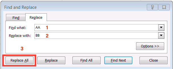
1. You need to enter the text that you want to find
2. Enter the text that you want that text to be replaced with.
3. Click on ‘Replace All’ and Excel will then search through all of the highlighted cells and replace the contents of all of the cells containing AA with BB.
If you’ve not got this quite right remember CTRL + Z will undo the changes you’ve just made!
Now… use these Excel tips and enjoy all of the time you save!
Author Bio:
Ben Richardson is a director of Acuity Training one of the UK’s learning providers of classroom based Excel training.


